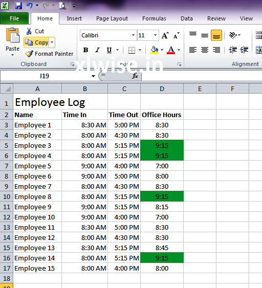
Have you ever felt the need to highlight different cells with different colors in Excel based on some criteria. If the answer is yes, this tutorial can help you for sure. The solution to your problem lies in "Conditional Formatting" functionality of Excel.
I will be taking a very simple example to demonstrate this. Imagine you have a report of employees with their Time-In and Time-out along with their office hours (Time-out - Time-In).
Now you want to highlight cells which have more than 9 hours in column D i.e Office hours. Select the cells on which you wish to define a rule
Click on "Conditional Formatting" and then "New Rule"
You will see a pop-up as below
Click on the second option "Format only cells that contain" ans choose the "greater than" value from the drop down as show below
Put the value "9:00" in the box and click on "Format"
You will see the following pop-up
You can choose the format you want to assign to the cells which satisfy the aforementioned rules. I am choosing to fill the cells with green color
Click on "OK" on this window
Click on "OK" on this window to apply the rule to selected cells
You can see that only the cells with values more than 9:00 are filled with green color. You can also define multiple rules on the same cell range or a different cell range too.


0 comments:
Post a Comment